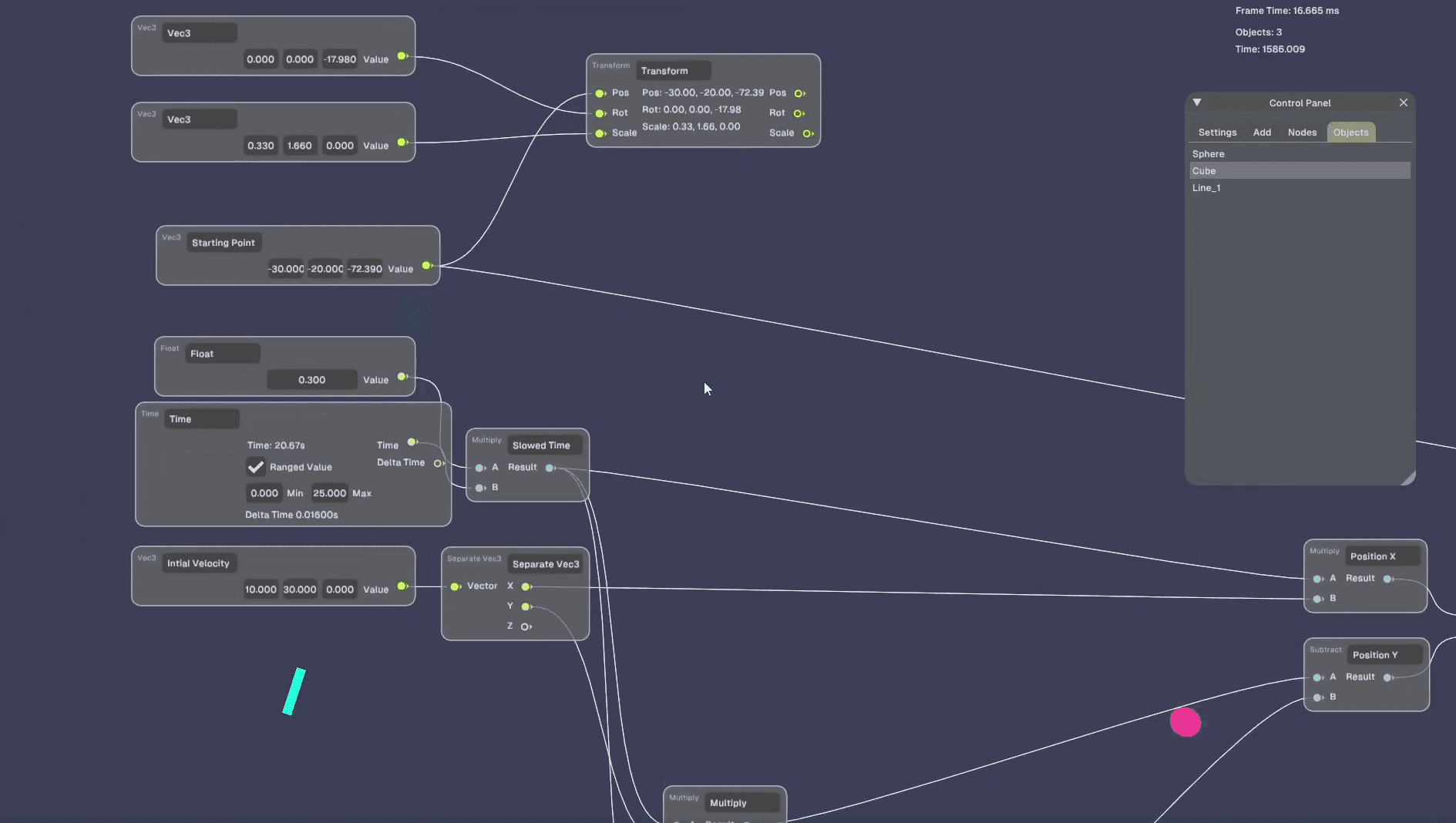
A small engine for looking at physics computed on the GPU. Vulkan does the rendering, the GPU does the compute, and a typed node graph sits in the middle so a simulation can be wired up without recompiling every time a constant changes. The first real workload is the hydrogen atom: give it (n, l, m) and it draws the orbital.
How it is put together
Rendering is Vulkan. SDL3 owns the window and input, volk loads the API, and shaders are written in Slang and compiled at runtime, so a shader edit is a restart and not a rebuild. The main scene layer is GPU driven: a compute pass builds the indirect draw commands, and the vertex work for lines, circles and orbital samples happens in compute shaders before anything reaches the graphics pipeline.
The heavy numerical work, sampling electron densities at the bandwidth roof, is CUDA and lives in its own repository, cuda-orbital-sampler, where it can be profiled properly. The engine is the place those samples get drawn.
Everything in the scene is a component. A tiny ECS holds Transform, MeshRenderer, LineRenderer, VolumeRenderer, Atom (the quantum numbers, validated so l < n and |m| <= l) and AtomVisualizer (how those numbers become geometry). Components draw their own inspector UI.
The node graph drives values
A typed node system (float, int, vec2 to vec4, mat4) with value, math, vector, object and graph nodes, drawn on top of imgui_node_editor. Node outputs bind to component properties, so a sine node wired into a transform is an animation and a constant node wired into an atom is a slider that changes the orbital. Projects save and load through a registry with JSON scene serialisation.
Status
Work in progress and it moves in bursts. The rendering path, node graph, saving and the atom components work. What it is building towards is the CUDA sampler feeding the visualizer directly rather than through dumps, and a proper simulation loop on the world layer. Built with CMake, C++23 and the Vulkan SDK; developed on Linux with Wayland.
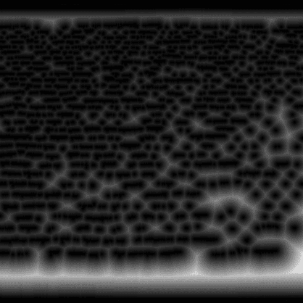
Batch image processing on the GPU: each grayscale image is thresholded into a site map, then an exact Euclidean distance transform is computed with NVIDIA NPP’s Parallel Banding Algorithm. Custom CUDA kernels handle the thresholding and the 8-bit visualisation on either side of the NPP call.
Pipeline
Load an 8-bit grayscale TIFF, copy it to pitched device buffers, run a CUDA kernel that turns pixels at or below the threshold into sites, compute the PBA+ distance transform so each pixel stores its Euclidean distance to the nearest site as float32, then normalise the field to 8 bits with an NPP max reduction and a second kernel. If an image has no pixels in range the threshold falls back to the image minimum, so every file still produces a distance field. A synthetic rectangle is processed first as a correctness check and its corner distance must match hypot(100, 200).
Results
One run on an RTX 2070 Super processed all 64 USC SIPI textures at 512x512 and 1024x1024 in a single execution. Distance-transform GPU time was about 32 ms for the batch; wall time including TIFF I/O was about 0.38 s. Scratch buffers are allocated once per resolution and reused across the batch, and the site map lives in a separate device image so the original can still be saved.

Given the quantum numbers (n, l, m) of a hydrogen orbital, draw millions of positions distributed exactly the way the electron would be found, each with its density. It is a tiny amount of maths per sample and one of the most bandwidth bound things I have written. The climb goes from a CPU loop to a kernel that sits at 77% of the card’s measured write roof.
The result first
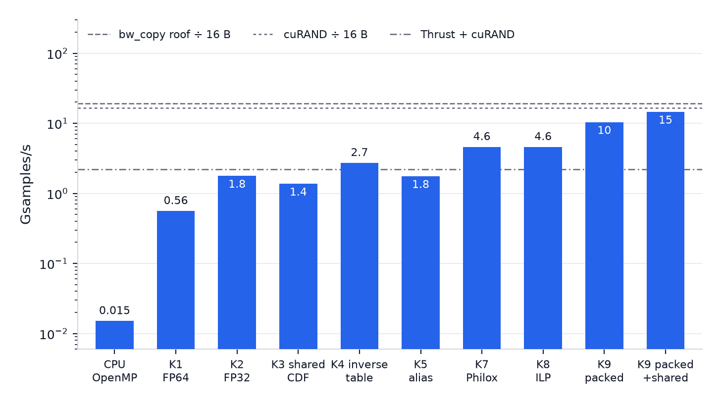
RTX 2070 Super Max-Q, SM clock locked at 1500 MHz, 8 million samples of the ground state, median of 20 runs after 3 warmups. The roof is the measured 305 GB/s copy bandwidth divided by the 16 bytes each sample writes. The CPU reference with 16 OpenMP threads manages 0.015 Gsamples/s. The first CUDA kernel, one thread per sample in FP64 with a binary search on a CDF and cuRAND XORWOW, reaches 0.56. FP32 takes it to 1.78, an inverse CDF table to 2.72, stateless Philox to 4.60, aligned 8 byte alias records to 10.39, and staging the draw arrays in shared memory lands at 14.60 Gsamples/s, 234 GB/s of payload.
The short version of why: for the first six kernels the random number state is 96 of the 112 bytes each sample moves through DRAM, and none of those bytes are the answer. Everything before the Philox kernel is rearranging the other 16.
How I worked
Every step follows the same loop. Predict before writing: each part opens with a hypothesis file, a claimed number, the arithmetic behind it against measured referees rather than spec-sheet figures, and a line below which the prediction counts as falsified. Write the kernel with device code split into small inline functions so the pieces can be tested on their own. Verify before measuring, with a CPU FP64 reference and a statistical gate: moments against closed forms, Kolmogorov Smirnov and chi square on the marginals, a fine window over the radial node of (3,1,-1) that catches the bug the inverse table introduces, and bit-exact determinism across launch geometries. The benchmark refuses to emit official numbers without the gate file and the SM clock lock.
Read the profiler: Nsight Compute and Nsight Systems reports are committed for every kernel with a quote sheet, so the stall names are traceable. Then a retro that states what the model got right and wrong, with the ratio of measured to predicted. Several predictions missed, some by a lot, and those misses are the article.
What the branches hold
Each branch is the repository as it stood at that step: cpu-baseline, naive-cuda, inverse-table, alias-method, endgame and packed-records, with main carrying everything. The CPU reference came first because the common implementation of this sampler has three quiet bugs and I wanted an oracle before touching the GPU. Shared memory for the search lost, because a dependent chain of loads does not care which SRAM it chains through. The inverse table landed exactly on the XORWOW bandwidth ceiling I had itemised, and also broke the radial node, which is what forced the alias method. Only then did the 48 byte RNG state become the obvious target, and shrinking the alias record to 8 bytes with the draw arrays in shared memory is where the final 3.2x comes from.